Translate this page into:
Comparative study of wavelet-ARIMA and wavelet-ANN models for temperature time series data in northeastern Bangladesh
⁎Corresponding author. k.hasancee@gmail.com (Khairul Hasan)
-
Received: ,
Accepted: ,
This article was originally published by Elsevier and was migrated to Scientific Scholar after the change of Publisher.
Peer review under responsibility of King Saud University.
Abstract
Time-series analyses of temperature data are important for investigating temperature variation and predicting temperature change. Here, Mann–Kendall (M–K) analyses of temperature time-series data in northeastern Bangladesh indicated increasing trends (Sen’s slope of maximum and minimum yearly temperature at Sylhet of 0.03 °C and 0.026 °C, respectively, and a minimum temperature at Sreemangal of 0.024 °C) except for the maximum temperature at Sreemangal. The linear trends showed that the maximum temperature is increasing by 2.97 °C and 0.59 °C per hundred years, and the minimum, by 2.17 °C and 2.73 °C per hundred years at the Sylhet and Sreemangal stations, indicating that climate change is affecting temperature in this area. This paper presents an alternative method for temperature prediction by combining the wavelet technique with an autoregressive integrated moving average (ARIMA) model and an artificial neural network (ANN) applied to monthly maximum and minimum temperature data. The data are divided into a training dataset (1957–2000) to construct the models and a testing dataset (2001–2012) to estimate their performance. The calibration and validation performance of the models is evaluated statistically, and the relative performance based on the predictive capability of out-of-sample forecasts is assessed. The results indicate that the wavelet-ARIMA model is more effective than the wavelet-ANN model.
Keywords
Mann–Kendall test
ARIMA
ANN
Wavelet-ARIMA
Wavelet-ANN
1 Introduction
Temperature variations due to climate change are a major concern. According to the Fourth Assessment Report of the Intergovernmental Panel on Climate Change (IPCC) (2007), the global average surface temperature has increased by 0.74 (0.56–0.92 °C) from 1906 to 2005, which is greater than the corresponding increase of 0.6 (0.4–0.8 °C) for 1901–2000. The Intergovernmental Panel on Climate Change (IPCC) (2007), also noted that the mean annual temperature is expected to increase by 3.3 °C per century. Even if the mean annual rainfall remains unchanged, delays in the monsoon onset and unusual monsoon lulls due to variations in temperature may cause severe disruptions for agricultural activities, hydroelectric power generation and drinking water supplies. Food production is particularly sensitive to climate change because crop yields are directly dependent on climate conditions (temperature and rainfall patterns). In tropical regions, even small amounts of warming will lead to decreases in the amount of crops harvested. Higher temperatures will lead to large declines in cereal (e.g., rice, wheat) production around the world (Stern, 2007).
Currently, the average temperature in Bangladesh ranges from 17 °C to 20.6 °C during the winter and from 26.9 °C to 31.1 °C during the summer (Shahid, 2008). The average annual temperature in Bangladesh is expected to increase by 0.6–1.4 °C by 2050, and the average monthly temperatures may continue to rise. An increase in the winter temperature may reduce the environmental suitability for wheat, potatoes and other temperate crops that are grown in the Rabi season (November–April). In Bangladesh, both surface water and groundwater are required to support irrigation during the dry months. Increases in temperature may affect irrigation requirements for all growing seasons, including Rabi (November–April) and Kharif (May–October). Increases in temperature will increase irrigation demands by 200 mm3 in March alone. The production of Boro rice in the Sylhet region is more than 5000 kg/ha, but this value is expected to drastically decrease upon maximum and minimum temperature increases of 2 °C and 4 °C. For a 2 °C increase, the Boro rice yield will decrease by 3.2–18.7%, and for 4 °C, the yield will decrease by approximately 5.33–36.0% (Basak, 2010).
The non-parametric Mann–Kendall (M–K) test can be used to detect trends in time-series analyses (Hamed, 2008; Hamed and Rao, 1998; Yue et al., 2002; Yue and Wang, 2004; Shadmani et al., 2012). Miao et al. (2012) described the use of the rank-based Mann–Kendall (M–K) test to assess the significance of trends in time-series data. The authors performed a comprehensive review of the trend and periodicity of seasonal data from Beijing, China for 1724–2009. Linear regression analysis and the Mann–Kendall (M–K) test were applied to study rainfall trends.
Over the past years, ARIMA model has been widely used in predicting of geophysical as well as hydrological time series (Salas et al., 1980; Salas and Obeysekera, 1982; Mohammadi et al., 2006; Momani, 2009; Liming et al., 2013). However, it assumes that data are stationary and has a limited ability to capture non-stationarities and non-linearities in hydrol-climatic data (Nourani et al., 2008).
Most artificial neural network (ANN) applications in engineering are used for predictions, in which an unknown relationship exists between a set of input factors and an output (Shi, 2002). ANNs have become a valuable tool for modeling non-linear phenomena, such as temperature predictions (Şahin, 2012; Chenard and Caissie, 2008), rainfall predictions (French et al., 1992; Aksoy and Dahamsheh, 2009; Mandal and Jothiprakash, 2012; Farajzadeh et al., 2014), and groundwater level forecasts (Daliakopoulos et al., 2005; Yang et al., 2009).
Recently, wavelet transformation has shown excellent performance in hydrological modeling (Okkan, 2012a; Nourani et al., 2008) as well as in multiple atmospheric and environmental applications (Pal and Devara, 2012; Pal et al., 2014a,b). Wavelet transformation decomposes the main time series into subcomponents such that the decomposed data improve the performance of geophysical and hydrological prediction models by capturing useful information at various resolution levels (Karim, 2013; Okkan, 2012b; Okkan and Samui, 2012; Nourani et al., 2008, 2011).
The wavelet-based ARIMA model can achieve higher prediction accuracy than the conventional ARIMA model (Wei et al., 2011; Kriechbaumer et al., 2014; Szolgayová et al., 2014; Fard and Zadeh, 2014). Rahman and Hasan (2014) used wavelet transformation to improve existing forecasting models (such as ARIMA) to forecast climate time series (e.g., the humidity of Rajshahi).
Recently, the combined wavelet-artificial neural network (Wavelet-ANN) model has been widely used to forecast hydrological and hydrogeological phenomena (Solgi et al., 2014; Okkan, 2012a,b; Nourani et al., 2009). A non-stationary signal is decomposed into several stationary signals by a wavelet transform. Then, ANN is combined with the wavelet transform to improve the prediction accuracy (Zhou et al., 2008). Ramana et al. (2013) used a combination of the wavelet technique with an ANN to predict rainfall using monthly rainfall data from the Darjeeling rain gauge station and found that the wavelet neural network models performed better than the ANN models alone. Partal and Cigizoglu (2009) estimated Turkish daily precipitation data with a wavelet-ANN application using wavelet sub-series of various meteorological variables; the wavelet-ANN model provided a better fit than the conventional ANN model and a multi-linear regression model. Adamowski and Chan (2011) proposed a WA–ANN model based on coupling discrete wavelet transforms (WA) and ANNs for groundwater level forecasting and found that the WA–ANN model provided better forecasting accuracy than the conventional ANN model.
The present study aims at analyzing the trend and pattern of temperature to see the transient variations. It also develops an alternative method using wavelet technique to predict monthly maximum and minimum temperatures. A comparison between wavelet-ARIMA and wavelet-ANN is conducted to find out the best-fitted model.
2 Study area and data collection
Sylhet, the northeastern administrative division of Bangladesh, is located at 24.8917°N latitude and 91.8833°E longitude. Sreemangal, which is known as the “tea capital of Bangladesh”, is located at 24.3083°N 91.7333°E and is a upazila of the Maulvibazar district in the division of Sylhet. The northeastern part of Bangladesh is an interesting study area because of its natural resources, such as its tilas (small hills), which contain more than 150 tea gardens that are sensitive to heavy rainfall and temperature, and its nearly 400 haors (wetland ecosystem), which cover approximately 4450–25,000 square km, and its role in the regional ecosystem. The region supports diverse livestock as well as the general well-being of a growing population that depends on the wetland for their livelihood.
Monthly temperature data from the northeastern part of Bangladesh, including the Sylhet district and the neighboring Sreemangal district (Fig. 1), were collected from the Bangladesh Meteorological Department (BMD), which is the authorized government organization for meteorological activities in Bangladesh.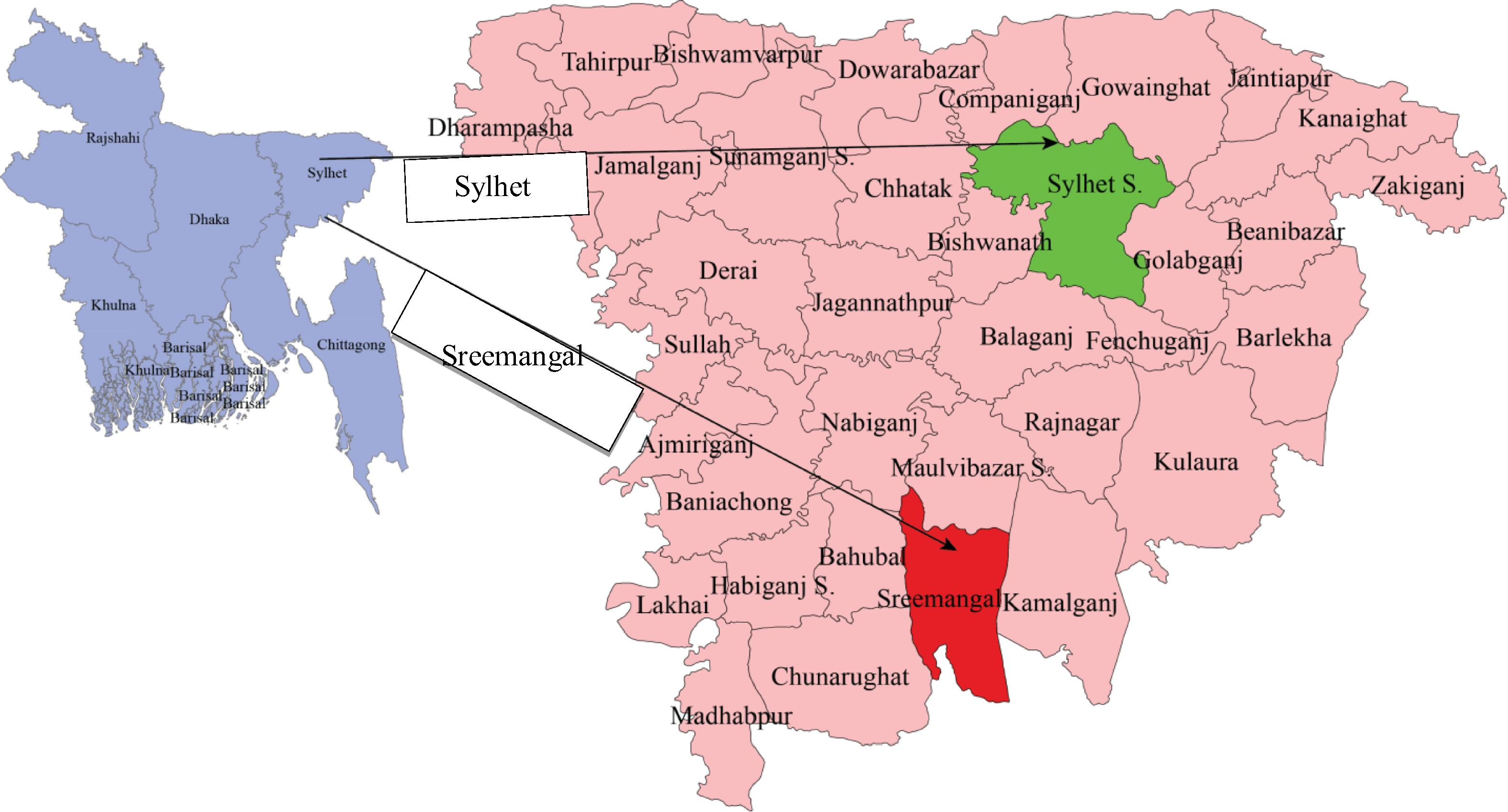
Locations of temperature stations.
3 Missing data treatment
The problem of handling missing data in an environmental time series is a serious issue in forecasting (Haworth and Cheng, 2012). In an environmental time series, missing data lead to several general problems for research and simulation. Missing data not only cause difficulties in process identification and parameter estimation but can also cause misinterpretations regarding the spatial and temporal variations of environmental indicators (Gnauck and Luther, 2005). To estimate missing data, this study applied three traditional geostatistical interpolation methods to the monthly maximum and minimum temperature data for the selected weather stations. The kriging, inverse distance weight (IDW) and nearest neighbor (NN) geostatistical interpolation techniques were employed to estimate missing points from the surrounding known values. Table 1 shows the performance measures root mean square error (RMSE) and accuracy, for the monthly maximum temperatures at the Sylhet station for the different methods. The results show that the RMSE is lowest for kriging and highest for IDW. The accuracy is also highest for kriging and lowest for IDW. Thus, IDW is not suitable for estimating the missing values. In contrast, kriging is appropriate for estimating missing values. Similar results were obtained for the maximum temperatures at Sreemangal and for the minimum temperatures at Sylhet and Sreemangal. Thus, we conclude that kriging is the best method for estimating missing data.
Year
Original (°C)
Kriging (°C)
IDW (°C)
NN (°C)
1970
34.4
36.59
36.96
36.7
1980
32.9
34.16
35.45
34.4
1990
35.3
35.52
35.24
35.7
2000
36.7
37.14
36.76
37.6
2010
35
36.01
36.91
36
Root mean square error
1.237
1.828
1.379
Mean absolute percentage error
2.981
4.197
3.538
Accuracy
97.02%
95.80%
96.46%
4 Methods
4.1 Statistical moment
For a monthly time series with a sample size of N, the statistical moments (mean, variance, skewness and kurtosis coefficient) are used in this study, which have been used in several studies (Beecham and Chowdhury, 2010; Rashid et al., 2014).
4.2 Trend analysis
There are two types of trend analysis methods; parametric methods and non-parametric methods. Non-parametric tests are more suitable than their parametric counterparts when the data do not meet the assumption of normality (Afzal et al., 2011). The non-parametric Mann–Kendall (M–K) test is widely used to analyze trends in climatological and hydrological time series (Yue and Wang, 2004).
The Mann–Kendall (M–K) test is commonly applied to assess the statistical significance of a trend. This test evaluates whether the outcome values tend to increase or decrease over time. The test statistic, S (score), is then computed as
Sen’s estimator has been used in this study to determine the magnitude of trends in hydro-meteorological time series. Sen’s method uses a linear model to estimate the slope of the trend (Salmi et al., 2002).
In the parametric method, a scatter plot of the dependent variable and the independent variable is constructed. A least-squares linear regression line is then superimposed on the plot.
4.3 Wavelet analysis
Wavelet analysis has become a popular tool due to its ability to reveal information within the signal in both the time and scale (frequency) domains (Nourani et al., 2008). This property overcomes the basic drawback of Fourier analysis, which is that the Fourier spectrum provides a comprehensive description of the properties of the non-stationary processes by yielding a mapping that is localized in frequency but global in time (Pal and Devara, 2012). Wavelet analysis is a mathematical procedure that transforms the original signal (especially in the time domain) into a different domain for analysis and processing (Dong et al., 2001). This model is suitable for non-stationary data, i.e., where the mean and autocorrelation of the signal are not constant over time. Most financial time-series as well as climatic time-series data are non-stationary; therefore, wavelet transforms are used for these types of data.
Morlet first considered wavelets as a family of functions constructed from the translations and dilations of a single function, which is called the “mother wavelet”. These wavelets are defined by Eq. (3)
The parameter ‘a’ is called the scaling parameter or scale, and it measures the degree of compression. The parameter ‘b’ is called the translation parameter, which determines the time location of the wavelet. If then the wavelet in ‘a’ is a compressed version (smaller support in the time domain) of the mother wavelet and primarily corresponds to higher frequencies. When then has a larger time width than and corresponds to lower frequencies. Thus, wavelets have time widths that are adapted to their frequencies, which is the main reason for the success of the Morlet wavelets in signal processing and time–frequency signal analysis.
The wavelet transform is implemented using a multi-resolution pyramidal decomposition technique. A recorded digitized time signal S(n) can be divided into its detailed cD1(n) and smoothed (approximation) cA1(n) signals using a high-pass filter (HiF-D) and a low-pass filter (LoF-D), respectively. Discrete wavelet transformation is the basic tool required for analyzing time series via wavelets and plays a role analogous to that of the discrete Fourier transformation in spectral analysis (Percival and Walden, 2000). The discrete wavelet transform (DWT) is based on sub-band coding and yields a fast computation of the wavelet transform. It is easy to implement and reduces the required computation time and resources. The dyadic decomposition can be implemented in a real data set
, where the scale parameter ‘a’ is represented in the form of
and the translation parameter ‘b’ is represented by
, where j,
. The discrete wavelet function can be expressed as
4.4 ARIMA model
The autoregressive integrated moving average (ARIMA) method can be used to identify complex patterns in data and to generate forecasts (Box and Jenkins, 1976). An ARIMA model predicts a value in a response time series as a linear combination of its own past values (Mudelsee, 2014). ARIMA models can accommodate seasonality (Makridakis et al., 1998). ARIMA models involve a combination of three types of processes: (1) an autoregressive (AR) process, (2) differencing to strip the integration (I), and (3) a moving average (MA) process. The general form of the ARIMA (p, d, q) model is
4.5 ANN Model (NARX model)
A neural network can be used to predict future values of possibly noisy multivariate time-series based on past histories and can be described as a network of simple processing nodes or neurons that are interconnected to each other in a specific order to perform simple numerical manipulations (Adamowski and Chan, 2011).
The NARX (nonlinear autoregressive network with exogenous inputs) model is based on the linear ARX (autoregressive with exogenous input) model, which is commonly used in time-series modeling. The defining equation for the NARX model is
4.6 Coupled wavelet and ARIMA (wavelet-ARIMA model)
Noise in the time-series data will significantly affect the accuracy of the forecast because ARIMA methods cannot handle non-stationary data without preprocessing the input data (Shan et al., 2014). To solve this problem, a wavelet denoising-based model is proposed.
When conducting wavelet analysis, the selection of the optimal number of decomposition levels is one of the keys to determine the performance of model in the wavelet domain. To select the number of decomposition levels, the following formula is used (Wang and Ding, 2003):
-
Step 1:
The wavelet transformation, which is a Daubechies-5 type and a decomposition level 3, is applied. Application to the series Yt (t = 1, 2,…, T) results in 4 series, which are denoted by A3t D3t, D2t and D1; t = 1, 2,…, T. WT (Yt; t = 1, 2,…, T) = {A3t, D3t, D2t, D1t: t = 1, 2,…, T}.
-
Step 2:
The series is reconstructed by removing the high-frequency component, using the wavelet denoising method.
-
Step 3:
The appropriate ARIMA model is applied to the reconstructed series to forecast the test series.
4.7 Coupled wavelet and ANN (wavelet-ANN) model
A wavelet-ANN model was constructed in which the subseries at time t are used as the inputs of the ANN and the denoised time series at time t is the output of the ANN network. The data set was then loaded and divided into two parts: training data (first 528 values of each data set) and testing data (subsequent 144 values of each data set). Tapped delay lines were used for both the input and the output, so the training began with the next data point of the tapped delay line. A two-layer series–parallel NARX network was created using the function narxnet.
The Levenberg–Marquardt (LM) algorithm was utilized to train the ANN models because it has been shown to be fast, accurate, and reliable (Adamowski and Karapataki, 2010). To identify the optimal number of hidden neurons, a trial and error procedure was initiated with two hidden neurons, and the number of hidden neurons was increased to 20 with a step size of 1 in each trial (Matarneh et al., 2014; Okkan, 2012a; Ramana et al., 2013). For each set of hidden neurons, the network was trained in batch mode to minimize the mean square error of the output layer. To identify overfitting during the training, a cross validation step was performed by evaluating the efficiency of the fitted model. The training was stopped when there was no significant improvement in the efficiency, and the model was then used for its generalization properties (Ramana et al., 2013).The trainlm function was used for training, and data were randomly divided for training, validation and testing. The toolbox function (closeloop) was used to perform an iterated prediction of the testing data (144 time steps).
4.8 Comparison of model performance
Model performance was assessed using root mean square error (RMSE), percent of bias (PBIAS) and index of agreement (d). Root mean square error (Singh et al., 2005) is an estimate of the standard deviation of the random components in the data, and the best model has a minimum RMSE. The percent of bias (Gupta et al., 1999) measures the average tendency of the simulated data to be larger or smaller than the observed counterparts. The optimal PBIAS value is 0.0, and low values indicate accurate model simulations. The index of agreement (Willmott, 1981) measures the degree of model forecast error and varies from 0 (no correlation) to 1 (perfect fit).
4.9 Programs used
In this study, missing data treatment was conducted using Golden Surfer software (version 10.1.561). Statistical trend and ARIMA model were conducted using R software packages (R-3.1.2). Wavelet analysis has been carried out using MATLAB software package. A Levenberg–Marquardt (LM) algorithm based ANN model was prepared using a MATLAB code (MATLAB, 2013).
5 Results and discussion
Wavelet transformation decomposed the time series into time–frequency space, enabling the identification of both the dominant modes of variability and how those modes vary with time. Fig. 2 shows the wavelet analysis of monthly maximum temperature of Sylhet. It identified significant variability (at the 95% confidence level) at an 8–16-month period from 1957 to 2012. The global wavelet spectrum provided two significant peaks above the 95% confidence level at 4–8-month and 8–16-month periods, respectively. Fig. 3 shows the wavelet decomposition of the maximum temperature signal for the Sylhet station. The signal wavelet is reconstructed using the approximation-and-detail process described above, and wavelet denoising is performed. Figs. 4 and 5 show the denoised signals of the maximum and minimum temperatures at the Sylhet station, respectively. The red lines indicate the original signals, and the black lines indicate the denoised signals. Outliers and noise are removed from the denoised signal, but the trend is the same as in the original series; this is the main mechanism of wavelet denoising.
Wavelet analysis of monthly maximum temperature of Sylhet. The thick curved black line in the wavelet power spectrum represents the cone of influence (COI). The dashed line in the global wavelet spectrum shows the 95% confidence level. The strength of power (%) in the contour image in the wavelet power spectrum is labeled by color (right corner) (MATLAB, 2013).
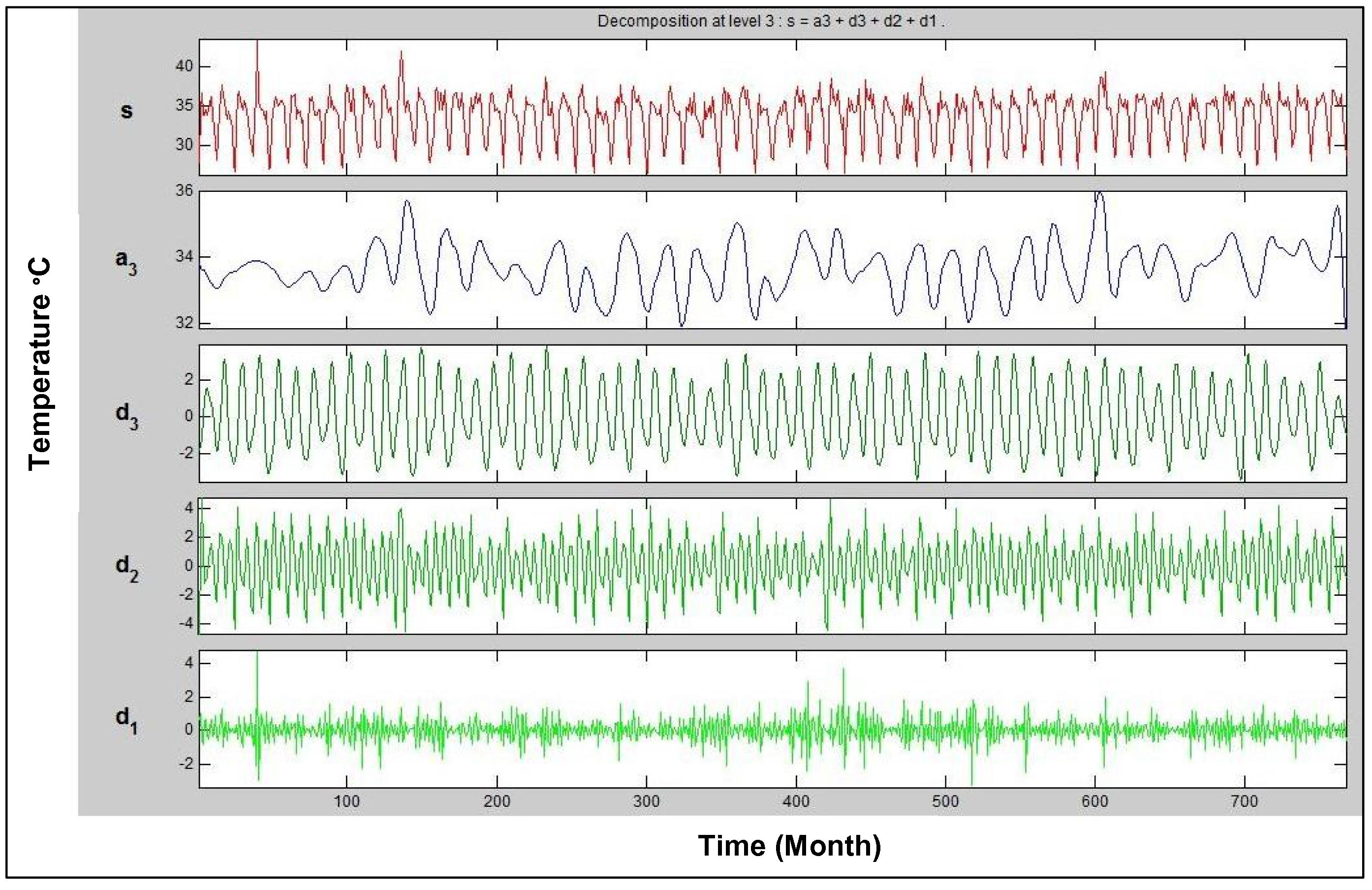
Wavelet decomposition of maximum temperature signal at Sylhet.
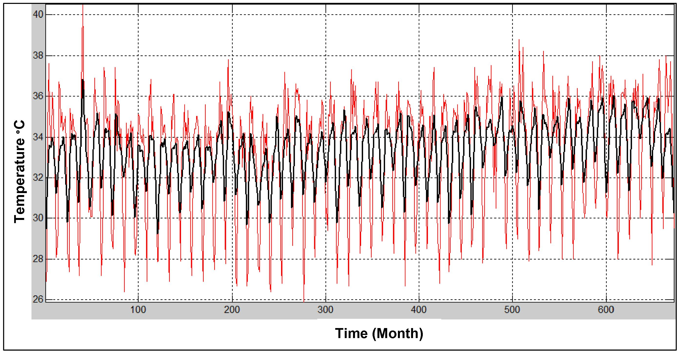
Wavelet de-noised signal of maximum temperature at Sylhet.
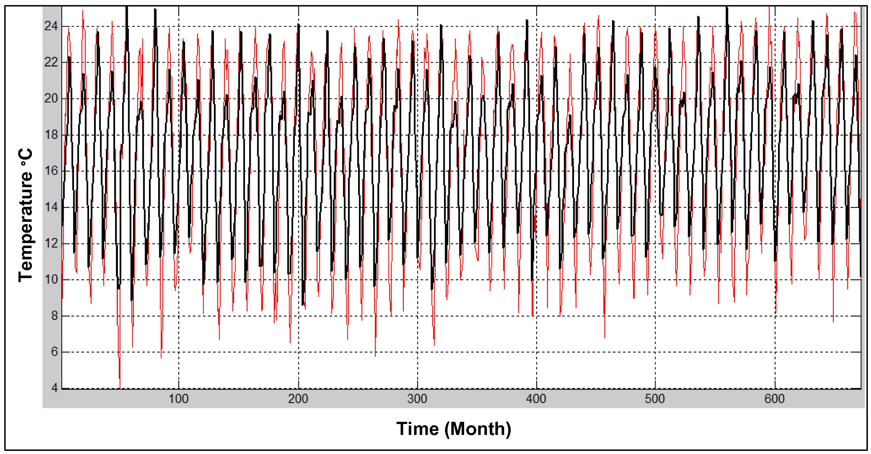
Wavelet de-noised signal of minimum temperature at Sylhet.
The augmented Dickey–Fuller (ADF) test was applied to test the unit root in the denoised maximum and minimum temperature series of the selected stations for different situations, such as in the presence of a drift, a drift and a linear trend, and no drift and a linear trend. Table 2 presents the ADF unit root test results for the original and 1st differenced series. The autocorrelation function (ACF) and partial autocorrelation function (PACF) are used to identify the order of the tentative model. The correlogram shows that the ACF has significant spikes at several lags, which display a periodic order over 12 months due to seasonal effects. The PACF also has significant spikes at several lags. Thus, the model may be a seasonal autoregressive integrated moving average (SARIMA) model. The least squares method is applied to estimate the parameter of the time series. For the Sylhet maximum temperature series, the final candidate model for estimating the parameter is SARIMA (3, 1, 3) (1, 1, 1)12. The estimated values, standard error, t-statistic and p-values for the SARIMA (3, 1, 3) (1, 1, 1)12 model are shown in Table 3. All coefficients for the estimated model are significant at the 5% level of significance. The R2 value of the estimated model is 0.903, indicating that approximately 90.3% of the variation in the monthly maximum temperature can be explained by the estimated previous lag value and the lagged error terms. The R2 and adjusted R2 values suggest the goodness of fit of the model. The autocorrelation was evaluated using the Durbin–Watson (D–W) test, and the results suggest that the estimated coefficients are free from autocorrelation problems because the D–W value is approximately 2. The minimum values of the Akaike information criterion (AIC), Schwarz information criterion (SC) and Hannan–Quinn criterion (H–Q) are also satisfactory. The correlogram and Q-statistics show that there are no significant spikes in the ACFs or PACFs (Fig. 6), which indicates that the residuals of this SARIMA model are white noise. There are no other significant patterns in the time series, and no other AR (p) and MA (q) terms need to be considered. Fig. 7 also shows that the histogram pattern of the maximum temperatures at Sylhet follows a normal distribution. Thus, the residuals are normally distributed. Fig. 8 shows that the fitted values nearly match the actual values and that the residuals do not vary significantly; thus, the fit is good. Hence, the final wavelet-ARIMA models for the selected variables were chosen.
Station
Include in test equation
Original series
1st differenced series
ADF statistic
p-value
ADF statistic
p-value
Sylhet maximum temperature
Drift
−2.369
0.151
−12.355
0.000
Drift and linear trend
−3.059
0.117
−12.365
0.000
None
0.089
0.711
−12.359
0.000
Variable
Coefficient
Std. error
t-Statistic
p-Value
AR(1)
0.111
0.038
2.903
0.004
AR(2)
−0.144
0.037
−3.939
0.000
AR(4)
−0.559
0.033
−16.720
0.000
SAR(24)
0.076
0.033
2.327
0.020
MA(1)
0.683
0.042
16.274
0.000
MA(2)
0.740
0.035
21.308
0.000
MA(3)
0.537
0.038
14.180
0.000
SMA(12)
−0.973
0.004
−233.814
0.000
R-squared
0.903
Adjusted R-squared
0.902
Akaike info criterion
−1.223
Durbin–Watson stat
1.997
Schwarz criterion
−1.167
Hannan–Quinn criterion
−1.202
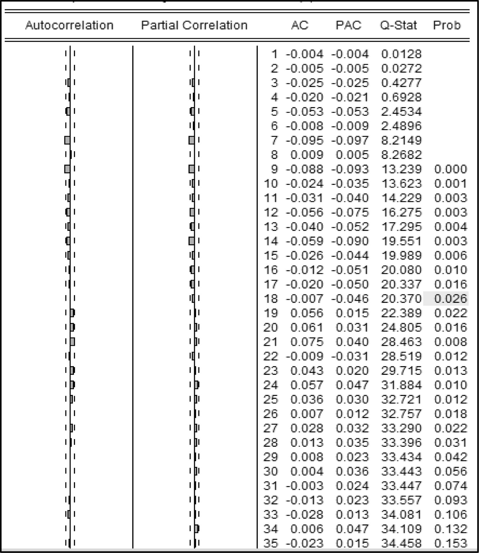
Correlogram-Q-statistics maximum temperature series at Sylhet.
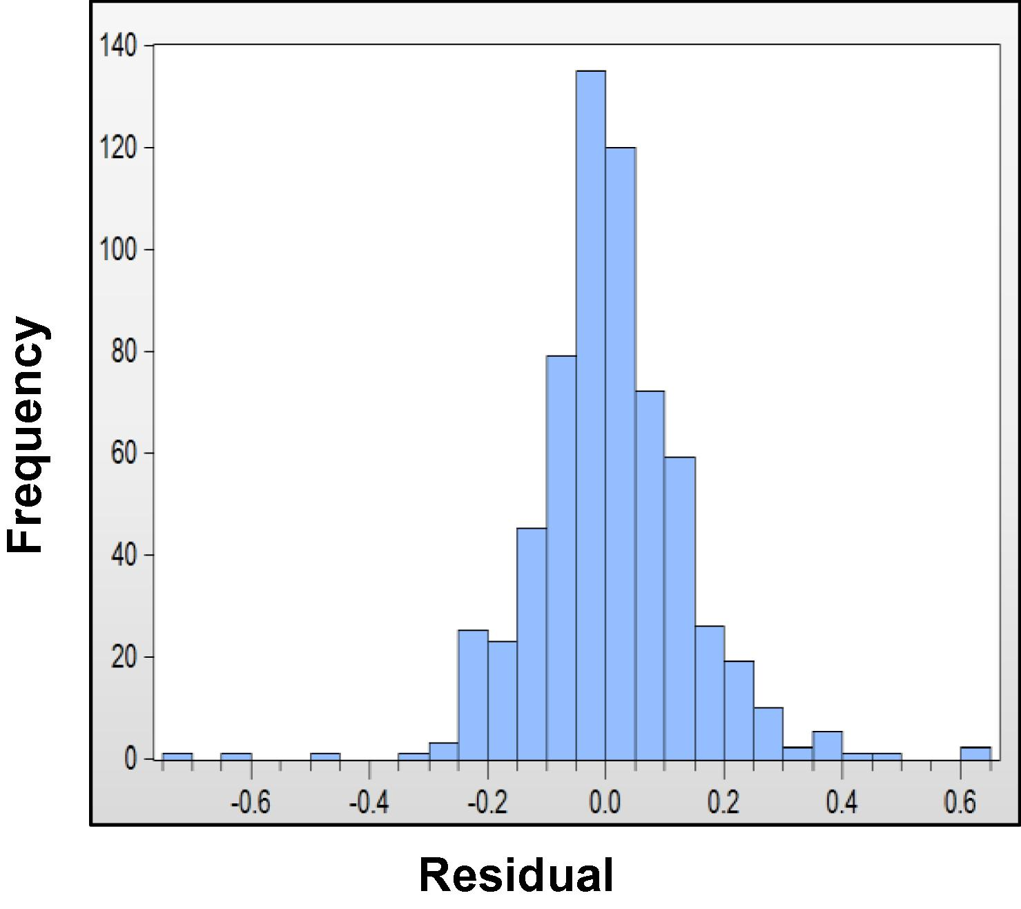
Histogram of maximum temperature at Sylhet.
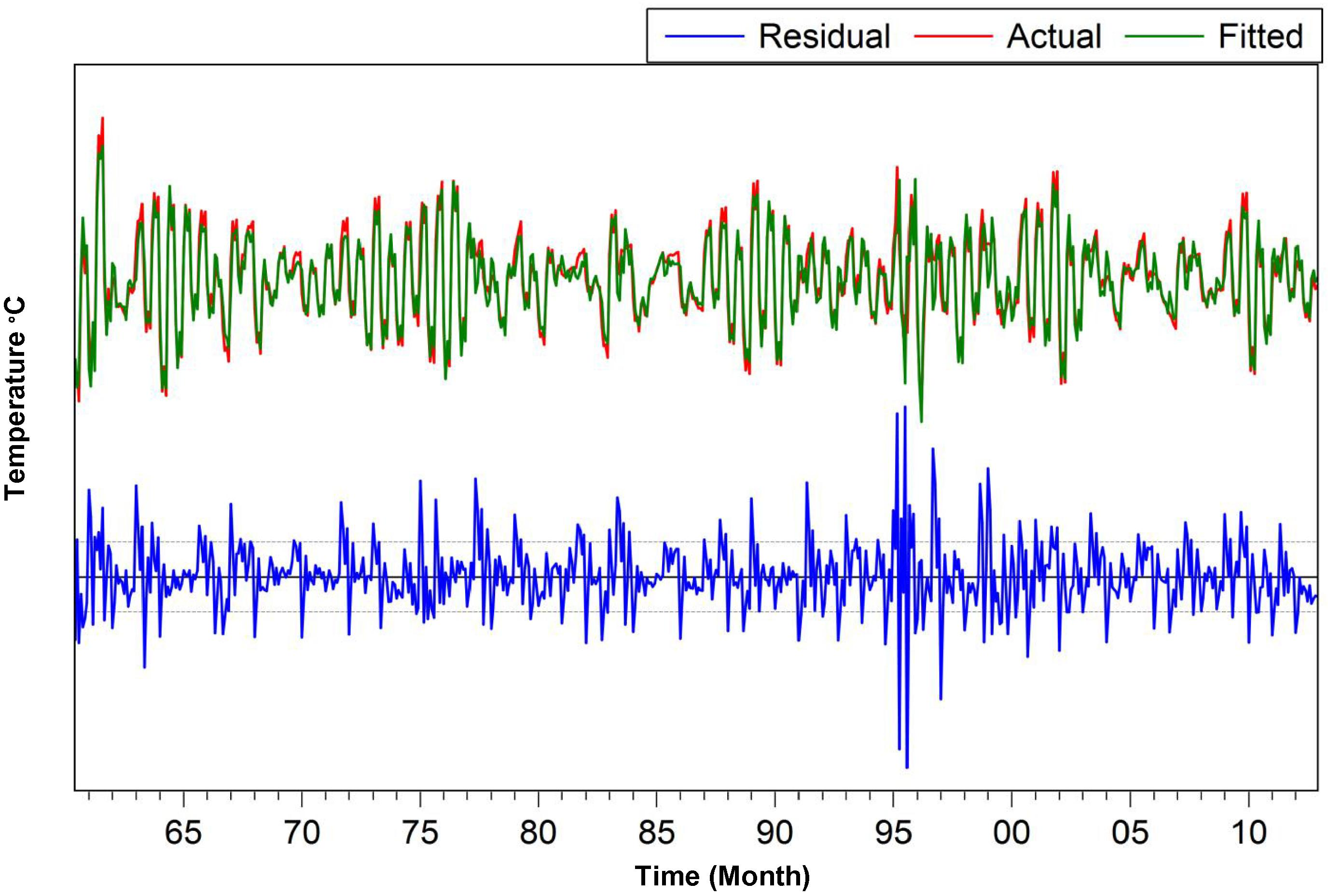
Actual, fitted, residual graph of maximum temperature at Syhet.
In this study, a Levenberg–Marquardt (LM) algorithm based on the ANN model was prepared using a MATLAB code (MATLAB, 2013).The original data were decomposed into different subseries, and the denoised time series was selected as the target of the ANN. The first 528 data points (January 1957–December 2000) were used to calibrate the model, and the last 144 data points (January 2001–December 2012) were used to test the model. After the network was trained, the network performance was verified using a neural network performance curve (Fig. 9), which shows that the validation set’s error curve reaches a minimum at different iteration numbers, indicating a good data division. The optimal number of hidden layers (10 for the maximum and minimum temperatures at Sylhet and 8 for the maximum and minimum temperatures at Sreemangal) was selected by trial and error. The number of epochs that are used to train was set to 1000. The training of ANN stopped when the error achieved 10−5 or when the number of epochs reached 1000. The R-value is greater than 0.9 (Fig. 10), which implies that the training data were well fit. The ANN was then applied to predict the testing data for the respective variables. Fig. 11 shows that the expected outputs and network predictions are similar.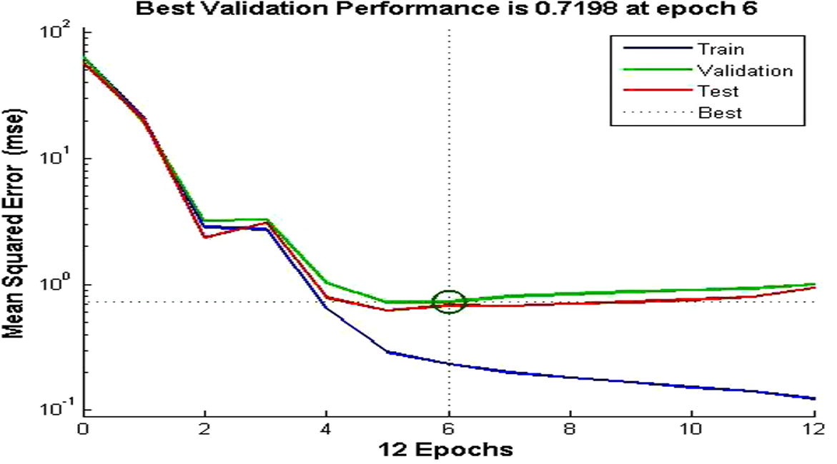
Neural network performance curve of maximum temperature at Sylhet.
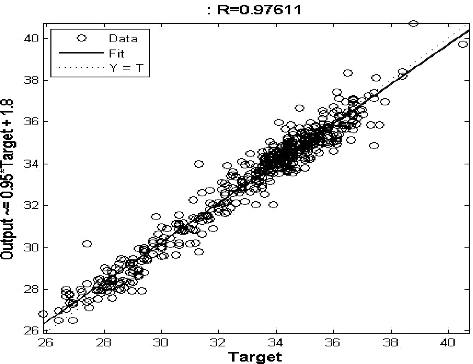
Regression value of NARX network during training of maximum temperature at Sylhet.
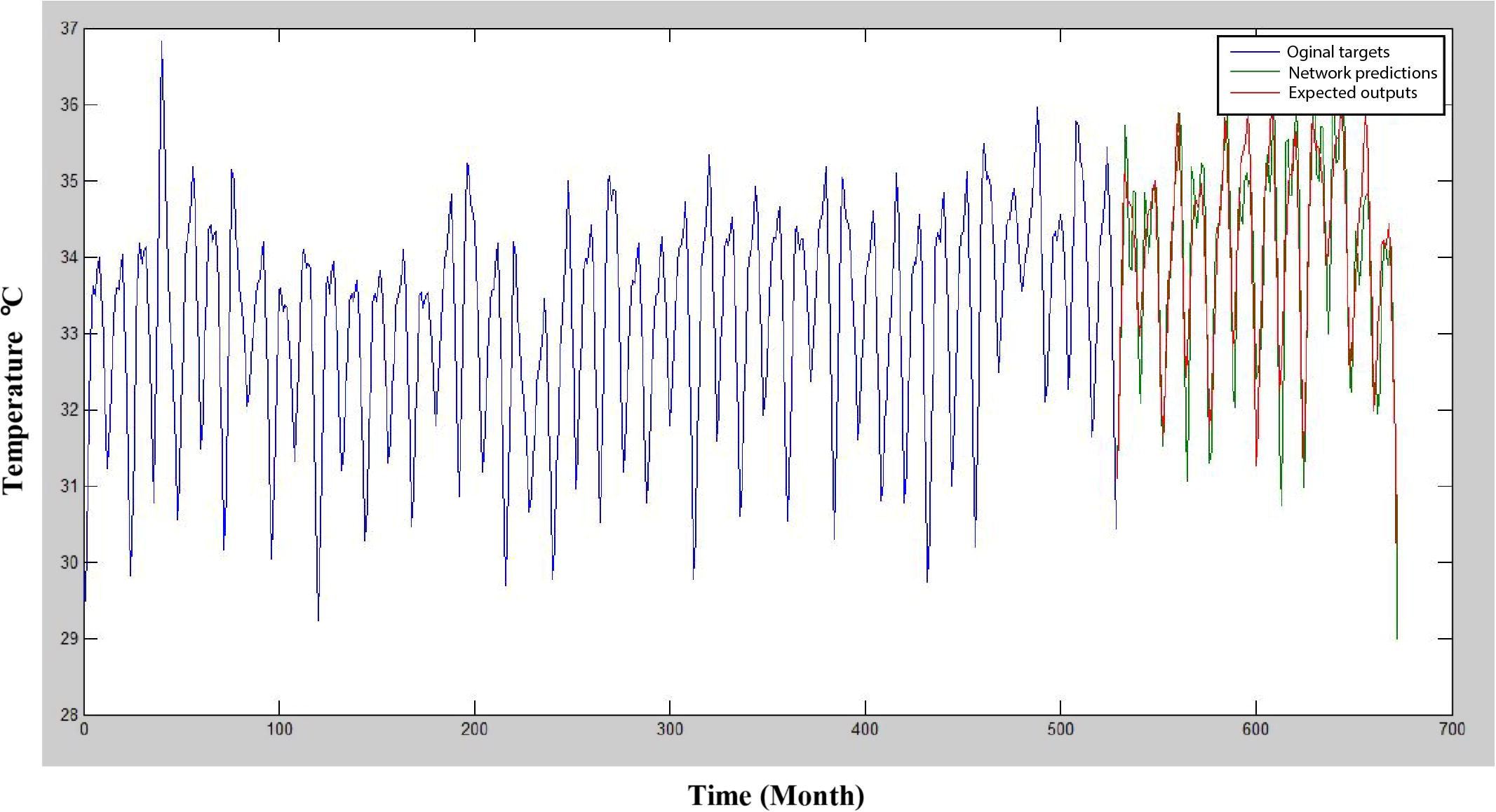
Prediction using NARX network of maximum temperature at Sylhet.
To determine the statistical moments, such as the mean, variance, skewness and kurtosis coefficient, data from the same month for all of the years at each station were considered (January in 1957–2012 from Sylhet form a series, February in 1957–2012 form a series, and so on). The monthly variations of the given statistical moments are shown in Figs. 12a–12d. The results show that the means of the maximum temperature at Sylhet and Sreemangal are nearly identical, and the means are constant from May to October. Although several small deviations are observed, the means of the minimum temperatures at Sylhet and Sreemangal are similar from April to October. The variances of the maximum and minimum temperatures of the respective stations are also small from July to September. Abrupt variations were observed from January to June and from October to December, especially for the minimum temperature at Sreemangal. The skewness coefficients of the minimum temperatures at Sylhet and Sreemangal are negative from March to November (i.e., the means are lower than the medians in the corresponding series), whereas the skewness coefficients of the maximum temperatures at Sylhet and Sreemangal are positive (i.e., the means are higher than the medians in the corresponding series), except for June and November. The variation of the kurtosis coefficient for the minimum temperature at Sreemangal is relatively high and has mostly positive values, whereas the kurtosis coefficient for the maximum temperature at Sylhet has no significant variation and is close to zero; i.e., the data have a nearly normal distribution. The minimum temperature curve for Sylhet and the maximum temperature curve for Sreemangal show that the variation is generally between 0 and 3, which indicates a normal distribution.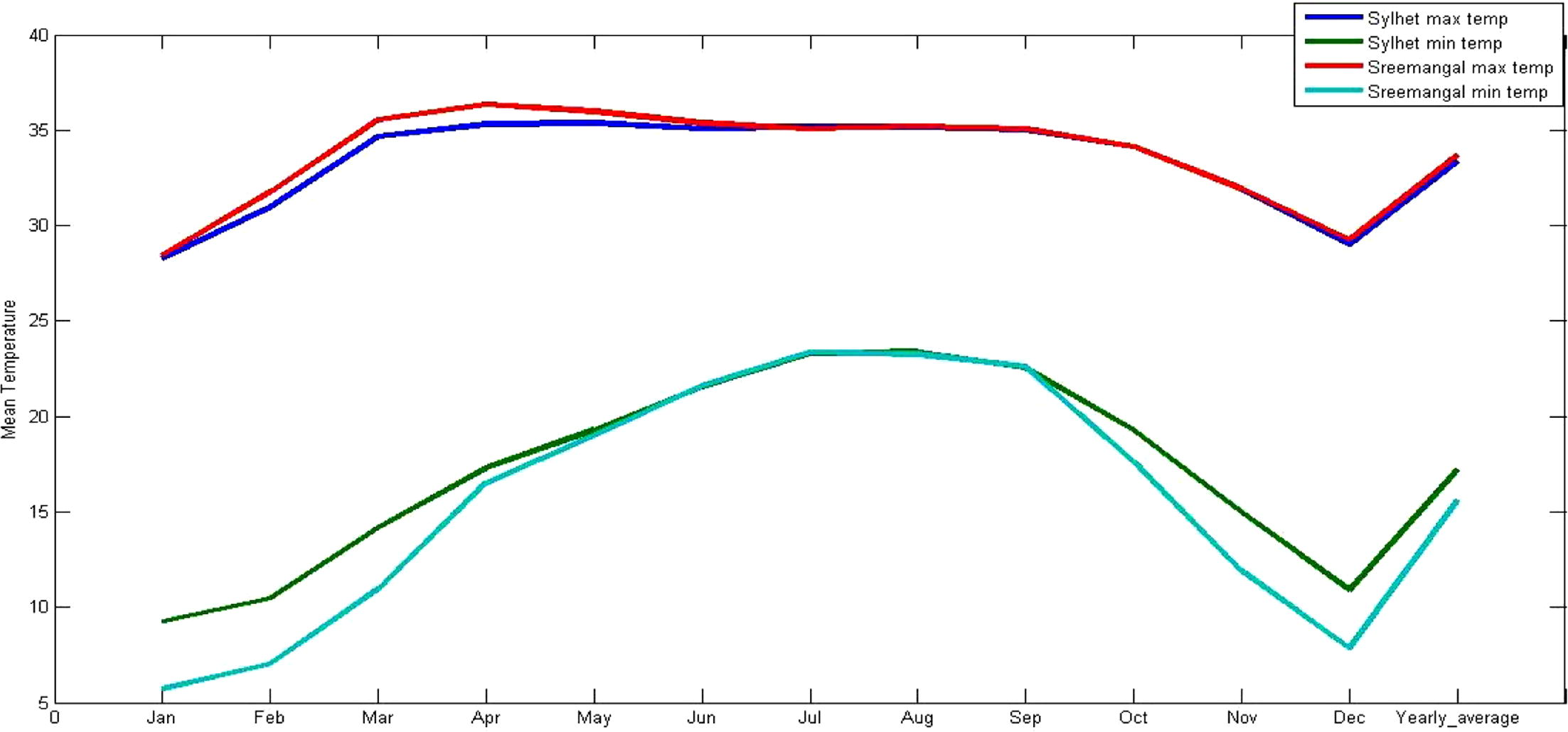
Monthly mean of the selected stations.
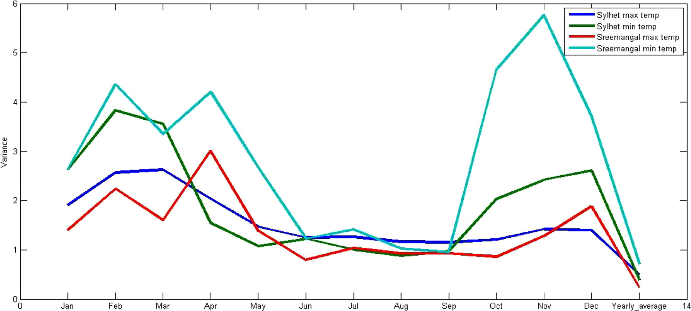
Monthly variance of the selected stations.
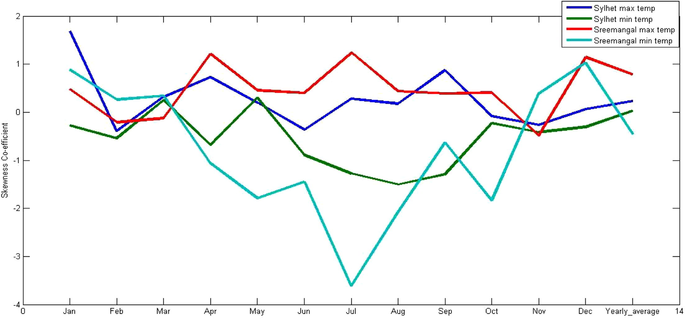
Monthly skewness of the selected stations.

Monthly kurtosis of the selected stations.
The results of the Mann–Kendall (M–K) tests for the monthly temperature data series from the two stations are shown in Table 4. The p-values of the Mann–Kendall (M–K) tests indicate trends in the maximum and minimum temperature data for Sylhet. There is no trend in the maximum temperature series for Sreemangal because the p-value (0.123) is greater than 0.05, but an increasing trend is observed in the minimum temperature data for Sreemangal. The annual maximum and minimum temperatures of the Sylhet station show an increasing trend (p-value < 0.0001). The maximum temperature at the Sreemangal station did not show a trend (p-value = 0.086), but the p-value for the minimum temperature (<0.0001) indicates an increasing trend. Sen’s slope, which refers to the slope of the trend, shows that the maximum and minimum temperatures at Sylhet had a trend of 0.002 ± 0.05 °C per month. The same trend is observed for the minimum temperatures at Sreemangal, whereas the maximum temperatures have no significant trend. The annual maximum temperature at Sylhet has a trend of 0.031 ± 0.05 °C per year, and the minimum temperature at Sylhet has a trend of 0.026 ± 0.05 °C per year, which is a clear indication of warming in this region. Similarly, the annual minimum temperature at Sreemangal has a trend of 0.024 ± 0.05 °C per year. The trends of the yearly maximum and minimum temperatures were analyzed for each station using linear regression analysis. A summary of the trend analysis is presented in Table 5 and indicates increasing trends for the yearly maximum and minimum temperatures at both the Sylhet and Sreemangal stations. The maximum temperatures at the Sylhet station have a high rate of increase (2.970.024 ± 0.05 °C per hundred years), whereas the Sreemangal station has a comparatively small rate of increase (0.59 °C per hundred years). Increasing trends for the yearly minimum temperature are observed at both stations, with rates of 2.17 °C per hundred years and 2.73 °C per hundred years for the Sylhet and Sreemangal stations, respectively.
Parameter
Station
Sen’s Slope
Kendall’s τ
p-value (two tailed test)
alpha, ɑ
Test interpretation
Maximum temperature
Sylhet
0.002
0.137
<0.0001
0.05
Trend in series
Sreemangal
6.54E-4
0.037
0.123
0.05
No significant trend in series
Minimum temperature
Sylhet
0.002
0.055
0.032
0.05
Trend in series
Sreemangal
0.002
0.060
0.013
0.05
Trend in series
Yearly-average maximum temperature
Sylhet
0.031
0.490
<0.0001
0.05
Trend in series
Sreemangal
0.005
0.147
0.086
0.05
No significant trend in series
Yearly-average minimum temperature
Sylhet
0.026
0.416
<0.0001
0.05
Trend in series
Sreemangal
0.024
0.407
<0.0001
0.05
Trend in series
Station
Yearly maximum temperature
Yearly minimum temperature
% of increasing rate(°C)
Climate line (°C)
% of increasing rate (°C)
Climate line (°C)
Sylhet
2.97
32.49
2.17
16.57
Sreemangal
0.59
33.49
2.73
14.73
According to WMO (World Meteorological Organization), the regional climatic scenario is changed after each 50 km distance. As the distance from Sylhet and Sreemangal is 81.4 km, this difference in geographic location is expected to influence the annual trend of temperature of this area. The magnitude of temperature at different stations varied between 0 and 0.26% of the normal annual temperature per year (IWFM, 2013). It was also found that the northern part of the country has a higher rate of increase in mean temperature compared to the mid-western and eastern hilly regions (IWFM, 2013). In our study, the difference between the trend of maximum temperature of Sylhet and Sreemangal is 0.026 °C per year. Moreover, the difference between the trend of minimum temperature of Sylhet and Sreemangal is 0.002 °C per year.
The predictive capabilities of the wavelet-ARIMA and wavelet-ANN models were compared using RMSE, d and PBIAS. The in-sample forecast was produced using the maximum temperature data for Sylhet over 528 months between 1957 and 2000, and the remaining 144 months from 2001 to 2012 were used for the out-sample forecast. The same procedure was also used for the other variables. The in-sample forecast RMSE and out-sample forecast RMSE are presented in Fig. 13. The results show that for the maximum temperature data of Sylhet, the RMSEs of both the in-sample and out-sample data are lower than those of the wavelet-ANN approach. Similar results were obtained for the other variables. For good predictive capability, the PBIAS value should be close to zero, and the index of agreement should be close to 1. The PBIAS value for the denoised maximum temperature of Sylhet is 0.02, which is satisfactory, and the index of agreement is 0.96, which indicates a good predictive capability compared to the wavelet-ANN approach (PBIAS = 0.18 and d = 0.86). However, the significance of differences between residuals was evaluated using tests of the equality of two means. The averages of residuals for the in-sample forecast from wavelet-ARIMA and wavelet-ANN are 0.00891 and 0.05897, respectively. The corresponding averages for the out-sample forecast are 0.00028 and −0.0605, respectively. According to the test of equality of two means, the difference between residuals for the in-sample forecast is not significant (z-value = −0.026 < 1.96). The difference between the residuals for the out-sample forecast is also insignificant (z-value = 0.017 < 1.96).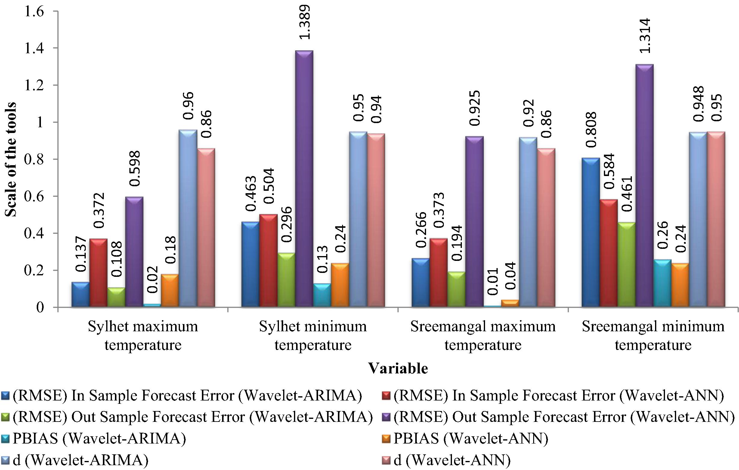
Comparison of predictive capability between wavelet-ARIMA and wavelet-ANN approaches.
Figs. 14a and 14b compare the original data with out-sample forecasted data for the denoised maximum temperature of Sylhet for both approaches. A visual inspection shows that the original data are more similar to the out-sample forecasted data for the wavelet-ARIMA approach than for the wavelet-ANN approach. This result might be due to the denoised signals that were used, in which the outliers were removed by the wavelet technique, whereas ARIMA uses the first and seasonal differences, which make the data stationary.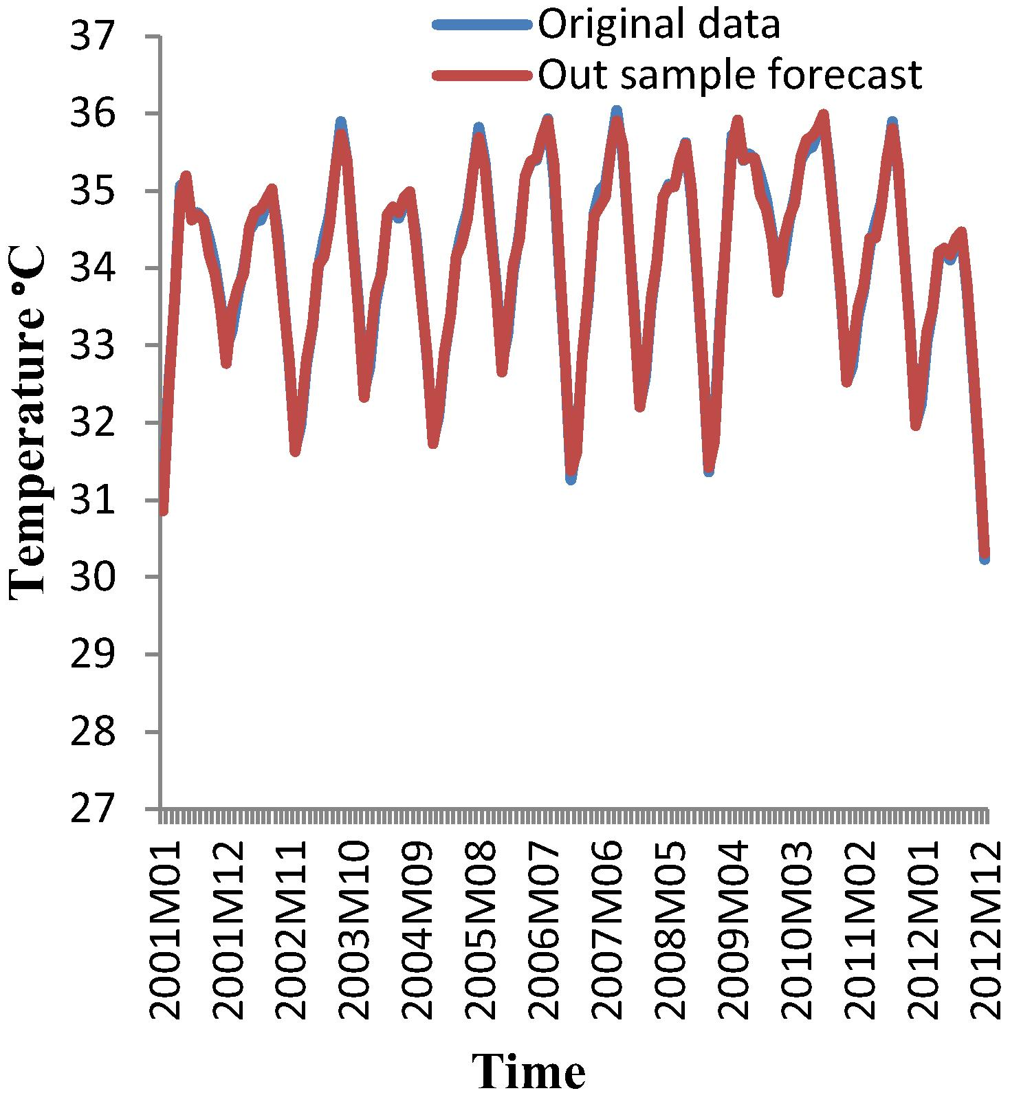
Out sample forecast for de-noised maximum temperature at Sylhet with wavelet-ARIMA (January 2001–December 2012).
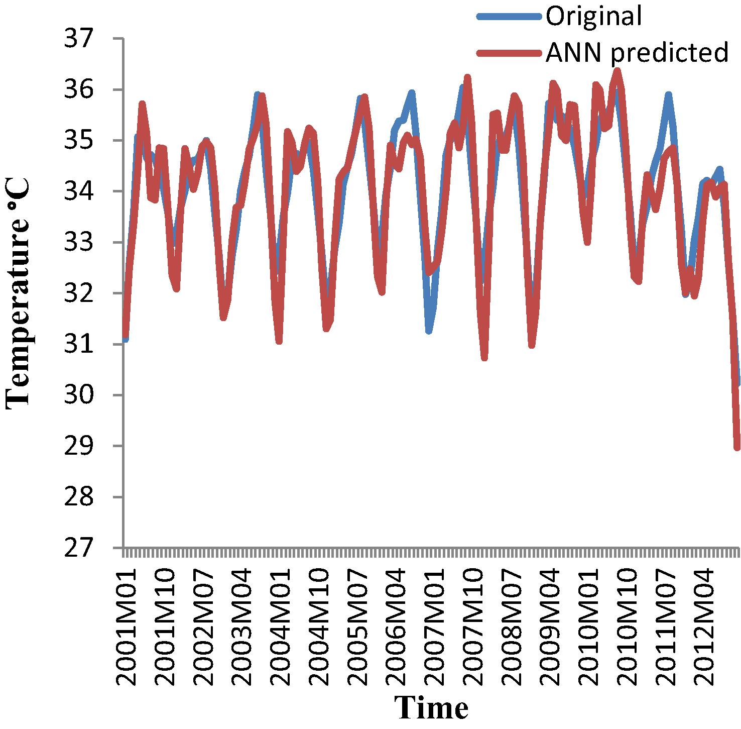
ANN predicted for de-noised maximum temperature at Sylhet with wavelet-ANN (January 2001–December 2012).
6 Conclusion
This study assessed the characteristics of temperature data and the predictive capabilities of two models for predicting temperatures in northeastern Bangladesh. The analysis indicates large temperature variations in this region. The results of this study can be summarized as follows. Mann–Kendall tests showed increasing trends in the maximum and minimum temperatures at Sylhet as well as in the minimum temperature at Sreemangal (Kendall’s τ = 0.137, 0.555, 0.060, respectively). Sen’s slope for the data was approximately 0.002 °C per month except for the maximum temperature at Sreemangal, which showed no significant trend (p-value = 0.123, which is greater than maximum threshold for the null hypothesis, ɑ = 0.05). The yearly maximum and minimum temperatures at Sylhet and the yearly minimum temperatures at Sreemangal showed increasing trends (Kendall’s τ = 0.490, 0.416, 0.407, respectively), but the maximum temperature at Sreemangal showed no significant trend (p-value = 0.086, which is greater than maximum threshold for the null hypothesis, ɑ = 0.05). The yearly maximum and minimum temperatures exhibited increasing trends of 0.031 °C and 0.026 °C per year at Sylhet, respectively, and the yearly minimum temperature at Sreemangal displayed an increasing trend of 0.024 °C. These trends may be a result of climate change in this region. The linear trends were positive in all cases, indicating that the temperature is increasing in this region. The temperature time series were smoothed using wavelet transformations, and the wavelet denoised signals were then used to fit the ARIMA model. For the monthly maximum and minimum temperatures at the Sylhet and Sreemangal stations, the ARIMA models were (3, 1, 3) (1, 1, 1)12, (2, 1, 3) (1, 1, 1)12, (3, 1, 5) (1, 1, 1)12 and (4, 1, 2) (1, 1, 1)12, respectively. Wavelet-ANN models were constructed using subseries of the denoised signals with the necessary verification. The predictive capability and accuracy (using the RMSE of the in-sample and out-sample data) were evaluated using the percent of bias (PBIAS) and the index of agreement (d) for the two models. The results indicate that the wavelet-ARIMA model is better for predicting temperatures in this region.
Acknowledgement
The authors would like to thank the Bangladesh Meteorological Department for providing support during this study.
References
- A wavelet neural network conjunction model for groundwater level forecasting. J. Hydrol.. 2011;407:28-40.
- [CrossRef] [Google Scholar]
- Comparison of multivariate regression and artificial neural networks for peak urban water-demand forecasting: evaluation of different ANN learning algorithms. J. Hydrol. Eng.. 2010;15(10):729-743.
- [CrossRef] [Google Scholar]
- Trends and variability in daily precipitation in Scotland. Procedia Environ. Sci.. 2011;6:15-26.
- [CrossRef] [Google Scholar]
- Artificial neural network models for forecasting monthly precipitation in Jordan. Stochastic Environ. Res. Risk Assess.. 2009;23(7):917-931.
- [CrossRef] [Google Scholar]
- Basak, J.K., 2010. Climate change impacts on rice production in Bangladesh: results from a model, Dhanmondi, Dhaka-1209, Bangladesh: Unnayan Onneshan-The Innovators. Available from: <http://www.unnayan.org/documents/Climatechange/climchange_impacts_rice_production.pdf>. (Last accessed 15.04.2015).
- Temporal characteristics and variability of point rainfall: a statistical and wavelet analysis. Int. J. Climatol.. 2010;30(3):458-473.
- [CrossRef] [Google Scholar]
- Wavelet-based nonlinear multiscale decomposition model for electricity load forecasting. Neurocomputing. 2006;70(1–3):139-154.
- [CrossRef] [Google Scholar]
- Time Series Analysis: Forecasting and Control. San Francisco: Holden-Day Inc.; 1976.
- Stream temperature modelling using artificial neural networks: application on Catamaran Brook, New Brunswick, Canada. Hydrol. Process.. 2008;22(17):3361-3372.
- [CrossRef] [Google Scholar]
- Groundwater level forecasting using artificial neural networks. J. Hydrol.. 2005;309(1–4):229-240.
- [CrossRef] [Google Scholar]
- Calculation of noise resistance by use of the discrete wavelets transform. Electrochem. Commun.. 2001;3(10):561-565.
- [CrossRef] [Google Scholar]
- Modeling of monthly rainfall and runoff of Urmia lake basin using “feed-forward neural network” and “time series analysis” model. Water Resour. Ind.. 2014;7–8:38-48.
- [CrossRef] [Google Scholar]
- A hybrid method based on wavelet, ANN and ARIMA model for short-term load forecasting. J. Exp. Theor. Artif. Intell.. 2014;26(2):167-182.
- [CrossRef] [Google Scholar]
- Rainfall forecasting in space and time using a neural network. J Hydrol.. 1992;137(1–4):1-31.
- [CrossRef] [Google Scholar]
- Missing Data in Environmental Time Series – A Problem Analysis. Informatics for Environmental Protection – Networking Environmental Information: Masaryk University Brno; 2005.
- Status of automatic calibration for hydrologic models: Comparison with multilevel expert calibration. J. Hydrol. Eng.. 1999;4(2):135-143.
- [CrossRef] [Google Scholar]
- Trend detection in hydrologic data: the Mann–Kendall trend test under the scaling hypothesis. J. Hydrol.. 2008;349(3–4):350-363.
- [CrossRef] [Google Scholar]
- A modified Mann–Kendall trend test for autocorrelated data. J. Hydrol.. 1998;204(1–4):182-196.
- [CrossRef] [Google Scholar]
- Non-parametric regression for space–time forecasting under missing data. Comput. Environ. Urban Syst.. 2012;36(6):538-550.
- [CrossRef] [Google Scholar]
- Climate change 2007: the physical science basis. In: Solomon, ed. Contribution of Working Group I to the Fourth Assessment Report of the Intergovernmental Panel on Climate Change. New York: Cambridge Univ. Press; 2007. p. :996.
- [Google Scholar]
- IWFM, 2013. Development of four decade long climate scenario & trend temperature, rainfall, sunshine & humidity. Comprehensive Disaster Management Program, Ministry Disaster Management and Relief, Dhaka. Available from: <http://reliefweb.int/sites/reliefweb.int/files/resources/291.%20Development%20of%20Four%20Decatde.pdf> (Last accessed 15.04.2015).
- Denoising the temperature data using wavelet transform. Appl. Math. Sci.. 2013;7(113):5821-5830.
- [CrossRef] [Google Scholar]
- A wavelet-support vector machine conjunction model for monthly stream flow forecasting. J. Hydrol.. 2011;399(1–2):132-140.
- [CrossRef] [Google Scholar]
- An improved wavelet–ARIMA approach for forecasting metal prices. Resour. Policy. 2014;39(1):32-41.
- [CrossRef] [Google Scholar]
- Time-series modeling and prediction of global monthly absolute temperature for environmental decision making. Adv. Atmos. Sci.. 2013;30(2):382-396.
- [CrossRef] [Google Scholar]
- Forecasting: Methods and Applications (third ed.). Wiley; 1998.
- Short-term rainfall prediction using ANN and MT techniques. J. Hydraul. Eng.. 2012;18(1):20-26.
- [CrossRef] [Google Scholar]
- Development of temperature-based weather forecasting models using networks and fuzzy logic. Int. J. Multimedia Ubiquitous Eng.. 2014;9(12):343-366.
- [CrossRef] [Google Scholar]
- MATLAB, 2013. The MathWorks Inc., Natick, MA.
- Long-term trend analysis of seasonal precipitation for Beijing, China. J. Resour. Ecol.. 2012;3(1):64-72.
- [CrossRef] [Google Scholar]
- Parameter estimation of an ARMA model for river flow forecasting using goal programming. J. Hydrol.. 2006;331(1–2):293-299.
- [CrossRef] [Google Scholar]
- Time series analysis model for rainfall data in Jordan: case study for using time series analysis. Am. J. Environ. Sci.. 2009;5(5):599-604.
- [CrossRef] [Google Scholar]
- Climate Time Series Analysis: Classical Statistical and Bootstrap Methods. Springer; 2014.
- A combined neural-wavelet model for prediction of watershed precipitation, Ligvanchai, Iran. J. Environ. Hydrol.. 2008;16(2):1-12.
- [CrossRef] [Google Scholar]
- A multivariate ANN-wavelet approach for rainfall-runoff modeling. Water Resour. Manage.. 2009;23(14):2877-2894.
- [CrossRef] [Google Scholar]
- Two hybrid artificial intelligence approaches for modeling rainfall–runoff process. J. Hydrol.. 2011;402(1–2):41-59.
- [CrossRef] [Google Scholar]
- Wavelet neural network model for reservoir inflow prediction. Sci. Iran.. 2012;19(6):1445-1455.
- [CrossRef] [Google Scholar]
- Using wavelet transform to improve generalization capability of feed forward neural networks in monthly runoff prediction. Sci. Res. Essays. 2012;7(17):1690-1703.
- [CrossRef] [Google Scholar]
- Modeling of watershed runoff using discrete wavelet transform and support vector machines. Int. J. Fresen. Environ. Bull.. 2012;21(12b):3971-3986.
- [Google Scholar]
- A wavelet-based spectral analysis of long-term time series of optical properties of aerosols obtained by lidar and radiometer measurements over an urban station in Western India. J. Atmos. Sol. Terr. Phys.. 2012;74(84–85):75-87.
- [CrossRef] [Google Scholar]
- Investigation of the atmospheric boundary layer depth variability and its impact on the 222Rn concentration at a rural site in France: Evaluation of a year-long measurement. J. Geophys. Res. Atmos.. 2014;120(2):623-643.
- [CrossRef] [Google Scholar]
- Impact of atmospheric boundary layer depth variability and wind reversal on the diurnal variability of aerosol concentration at a valley site. Sci. Total Environ.. 2014;496:424-434.
- [CrossRef] [Google Scholar]
- Prediction of daily precipitation using wavelet-neural networks. Hydrol. Sc. J.. 2009;54(2):234-246.
- [CrossRef] [Google Scholar]
- Wavelet Methods for Time Series Analysis. Cambridge University Press; 2000.
- Performance of wavelet transform on models in forecasting climatic variables. In: Computational Intelligence Techniques in Earth and Environmental Sciences. Netherlands: Springer; 2014. p. :141-154.
- [Google Scholar]
- Monthly rainfall prediction using wavelet neural network analysis. Water Resour. Manage.. 2013;27(10):3697-3711.
- [CrossRef] [Google Scholar]
- Statistical characteristics of rainfall in the onkaparinga catchment in South Australia. J. Water Clim. Change. 2014;6(2):352-373.
- [CrossRef] [Google Scholar]
- Feature extraction via multi-resolution analysis for short-term load forecasting. IEEE Trans. Power Syst.. 2005;20(1):189-198.
- [CrossRef] [Google Scholar]
- Modelling of air temperature using remote sensing and artificial neural network in Turkey. Adv. Space Res.. 2012;50(7):973-985.
- [CrossRef] [Google Scholar]
- ARMA model identification of hydrologic time series. Water Resour. Res.. 1982;18(4):1011-1021.
- [CrossRef] [Google Scholar]
- Applied Modeling of Hydrological Time Series. Colorado: Water Resources Publications; 1980.
- Detecting trends of annual values of atmospheric pollutants by the Mann–Kendall test and Sen’s slope estimates – the Excel template application MAKESENS. Helsinki: Finnish Meteorological Institute; 2002.
- Trend analysis in reference evapotranspiration using Mann–Kendall and Spearman’s Rho tests in arid regions of Iran. Water Resour. Manage.. 2012;26(1):211-224.
- [CrossRef] [Google Scholar]
- Spital and temporal characteristics of droughts in the Western part of Bangladesh. Hydrol. Process.. 2008;22:2235-2247.
- [CrossRef] [Google Scholar]
- Forecasting model for stock data based on new wavelet and conjugated-ARIMA combination model. J. Comput. Inf. Syst.. 2014;10(7):3023-3030.
- [CrossRef] [Google Scholar]
- Clustering technique for evaluating and validating neural network performance. J. Comput. Civil Eng.. 2002;16(2):152-155.
- [CrossRef] [Google Scholar]
- Hydrological modeling of the Iroquois River watershed using HSPF and SWAT. J. Am. Water Resour. Assoc.. 2005;41(2):361-375.
- [CrossRef] [Google Scholar]
- Forecasting daily precipitation using hybrid model of Wavelet-Artificial neural network and comparison with adaptive neurofuzzy inference system (Case Study: Verayneh Station, Nahavand) Adv. Civil Eng.. 2014;2014(2014):1-12.
- [CrossRef] [Google Scholar]
- Stern, N., 2007. Report of the Stern Review: The Economics of Climate Change. HM Treasury, London. ISBN: 9780521700801.
- Wavelet based deseasonalization for modelling and forecasting of daily discharge series considering long range dependence. J. Hydrol. Hydromech.. 2014;62(1):24-32.
- [CrossRef] [Google Scholar]
- Wavelet network model and its application to the predication of hydrology. Nat. Sci.. 2003;1(1):67-71.
- [Google Scholar]
- Wei, Y., Wang, J., Wang, C., 2011. Network traffic prediction based on wavelet transform and seasonal ARIMA model. In: Lecture Notes in Computer Science. 6677, 152–159. 8th, International Symposium on Neural Networks; Advances in neural networks – ISNN 2011: 8th International Symposium. Part III; 2011; Guilin, China. ISBN: 978-3-642-21110-2.
- Application and comparison of two prediction models for groundwater levels: a case study in Western Jilin Province, China. J. Arid. Environ.. 2009;73(4–5):487-492.
- [CrossRef] [Google Scholar]
- The Mann–Kendall test modified by effective sample size to detect trend in serially correlated hydrological series. Water Resour. Manage.. 2004;18(3):201-218.
- [CrossRef] [Google Scholar]
- Power of the Mann–Kendall and Spearman’s rho tests for detecting monotonic trends in hydrological series. J. Hydrol.. 2002;259(1–4):254-271.
- [CrossRef] [Google Scholar]
- The research of monthly discharge predictor-corrector model based on wavelet decomposition. Water Resour. Manage.. 2008;22(2):217-227.
- [CrossRef] [Google Scholar]


